Basic Functions

Functions

Basic functions are real-valued functions of a real variable. Basic functions can be represented by an analytical expression. At the elementary functions include rational functions, trigonometric functions, exponential and logarithmic functions and their inverse functions. In general, a function is a mapping between two quantities that accurately assigns to each element of one set is an element of the other.

Definition

A function f assigns to each element of a definition set D exactly one element of the target set Z. The element x ∈ D from the definition set is assigned to the target set element f(x).

$f : D \to Z, x \mapsto y$

Monotonously:

In mathematics, a function or sequence, which is only increasing or constant (i.e. never falling) with increasing function argument, is called monotonously increasing (or monotonously increasing or isotonous). Accordingly a function or sequence is called monotonously falling (antitonous), if it only becomes smaller or remains constant. If the values of the function or the elements of the sequence do not change anywhere, it is called constant. Strictly monotonously increasing (resp. strictly monotonously decreasing) are functions or sequences, which only become larger (smaller), but are nowhere constant.

Continuously:

A function is called continuously, if sufficiently small changes of the argument(s) result in arbitrary small changes of the function-value. This means especially, that there are no jumps in the function values.

Restricted:

A function is called restricted if the function values f(x) do not exceed an upper or lower limit. I.e., if f(x) ≤ M is valid for all real numbers x, then the function f is limited upwards. If M is the smallest number to which this applies, then M is the upper limit with respect to the function f. The analogous definition applies to the lower bound. If f(x) is greater than m for all x, then m is the lower bound.

Linear Function

Properties

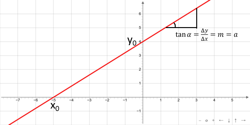
Linear functions are rational integral functions. They grow monotonically for a > 0 and fall monotonically for a < 0. The graph of a linear function is a straight line.

The linear function crosses the x-axis at x₀

$f (x_{0}) = 0$

$a \cdot x_{0} + b = 0$

$x_{0} = - \frac{b}{a}$

The linear function crosses the y-axis at y₀

$f (0) = y_{0} = b$

The slope m linear function is the parameter a.

$m = \tan α = \frac{Δ y}{Δ x} = \frac{f (x + Δ x) - f (x)}{Δ x} = a$

$f (x) = a \cdot x + b$

$with a, b \in R und a \neq 0$

Quadratic Function

Properties

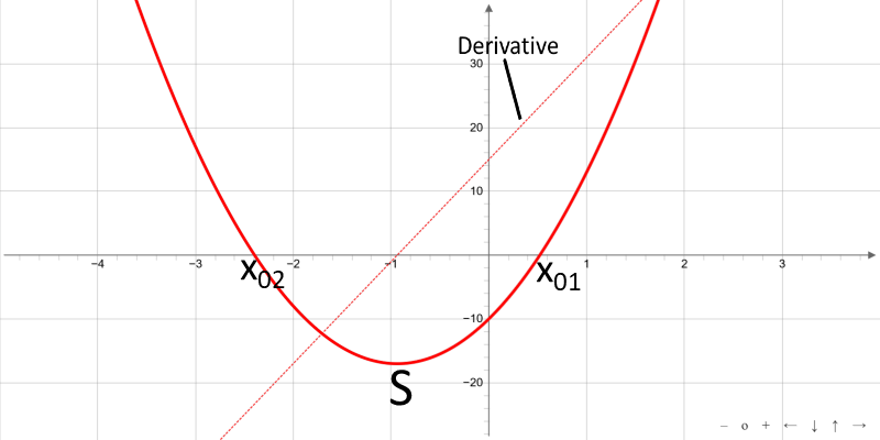
Quadratic functions are rational integral functions of second degree. The graph of a quadratic function is a parabola that opens upward or downward. For a > 0, the parabola opens upward, for a < 0 downward.

Roots

$x_{01, 02} = - \frac{p}{2} \pm \sqrt{{(\frac{p}{2})}^{2} - q}$

with

$p = \frac{b}{a} und q = \frac{c}{a}$

Vertex S

$S = (x_{s} y_{s}) = (- \frac{b}{2 a} c - \frac{c^{2}}{4 a})$

Derivative f′

$f' (x) = 2 a x + b$

Product representation

$f (x) = (x - x_{01}) (x - x_{02})$

$f (x) = a \cdot x^{2} + b \cdot x + c$

$with a, b, c \in R und a \neq 0$

Sine function

Properties

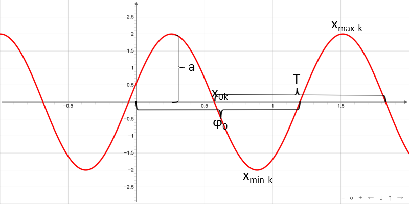
For a = b = 1 and c = 0, the ordinary sine function f (x) = sin (x) is available. It is a periodic function with period 2 π and the value range -1 ≤ f (x) ≤ 1.

The general sine function is shown by an affine transformation from the ordinary sine function. Stretching by a factor a in the direction of the y-axis, with the elongation factor 1 / b in the x-axis followed by parallel displacement in the direction of the x-axis to c / b.

Often, the parameters of the general sine function are named as follows:

$f (x) = A \sin (ω x + φ_{0})$

here A denotes the amplitude, ω is the angular frequency and φ₀, the phase shift.

Many processes in nature and technology that reflect the character of oscillations, can be described by the general sine function.

If the variable of the general sine function is the time t then it is called a harmonic oscillation

$f (t) = A \sin (ω t + φ_{0})$

with the phase shift φ₀, the amplitude A, the period T = 2 π / ω and the frequency f = 1 / T.

$f (x) = a \sin (b x + c)$

$with a, b, c \in R und a, b > 0$

Exponential function exp(x)

Properties

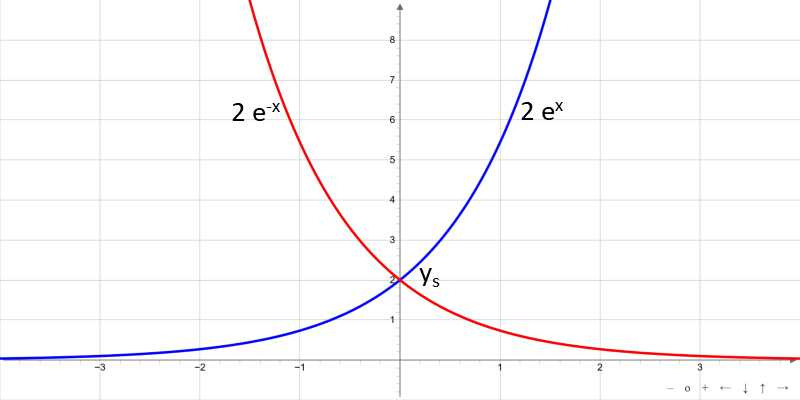
The exponential function is defined for all real numbers. The function has no zeros and no extremes. The function values are always positive and the function is for b > 0 monotonically increasing and monotonically decreasing for b < 0. The natural exponential function e^x is available for b = 1.

The addition theorem applies to the exponential functions:

$f (x_{1} + x_{2}) = f (x_{1}) + f (x_{2})$

The Inverse of the Exponential function f(x) = a^x is the Logarithm:

$f^{-1} (x) = \log_{a} (x)$

In the special case f(x) = e^x is the inverse the Logaritm naturalis:

$f^{-1} (x) = \log_{e} (x) = \ln (x)$

Applications

Description of organic growth with the initial value g₀ and growth constant c:

$g (t) = g_{0} e^{c t}$

Exponential growth differential equation

Description of a process of decay with m₀ initial size and λ the decay constant:

$m (t) = m_{0} e^{- λ t}$

Damped vibration with the damping constant R:

$f (t) = e^{- R t} \sin (ω t + φ_{0})$

$f (x) = c e^{b x}$

$with b, c \in R und b, c \neq 0$

$Setzt man a = c e^{b} so gilt:$

$f (x) = c e^{b x} = a^{x}$

Error function exp(-x²)

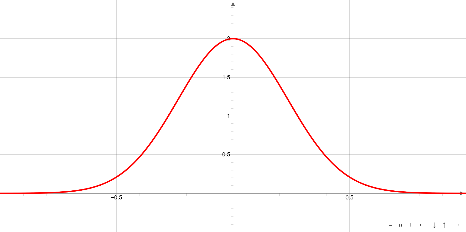
Properties

The function is defined for each real value and takes its maximum at x = 0 with y = b. The graph of the function is symmetrical about the y-axis.

Derivative:

$f' (x) = -2 a^{2} b x e^{- {(a x)}^{2}}$

Turning points:

$x_{w1} = \frac{1}{a \sqrt{2}}; y_{w1} = \frac{b}{\sqrt{e}}$

$x_{w2} = - \frac{1}{a \sqrt{2}}; y_{w2} = \frac{b}{\sqrt{e}}$

Turning point tangents:

${f'}_{w1} = a b \cdot \sqrt{\frac{2}{e}}$

${f'}_{w2} = - a b \cdot \sqrt{\frac{2}{e}}$

Special case

For

$b = \frac{1}{\sqrt{2 π}}; a = \frac{1}{\sqrt{2}}$

the function is the bell curve which describes the probability density of the normal distribution.

$f (x) = b e^{- {(a x)}^{2}}$

$with b > 0 und a \neq 0$

Normal distribution (Gaussian distribution)

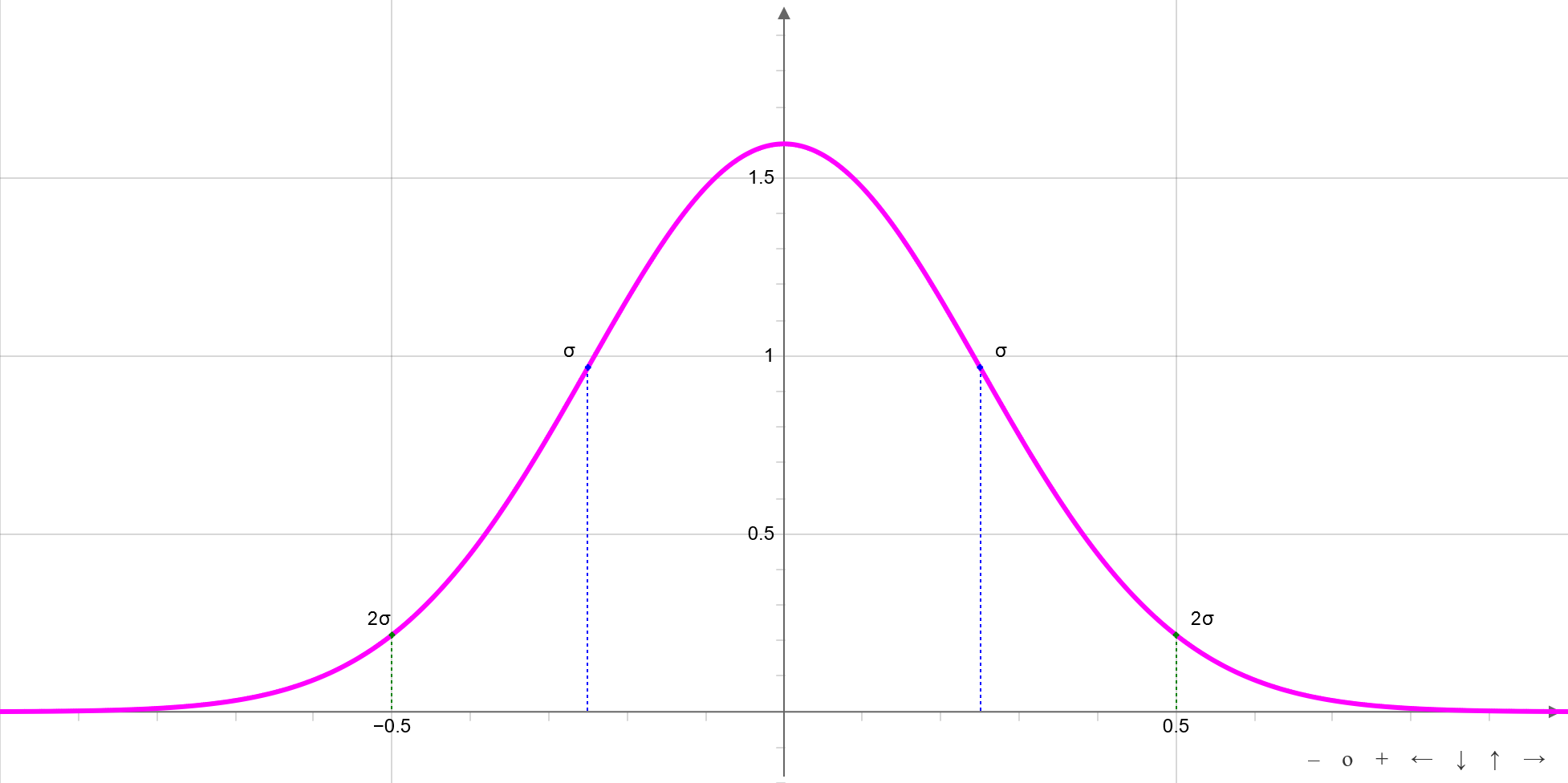
Properties

The image of the Gaussian distribution is a bell-shaped curve with the maximum and the symetric center at a. The σ parameter defines the spacing of the turning points from symetric center. If σ small, the bell curve is narrow and pointed. For large σ function is flat and wide.

$f (x) = \frac{1}{\sqrt{2 π} σ} e^{- \frac{1}{2} \frac{{(x - a)}^{2}}{σ^{2}}}$

$with σ > 0 und a \in R$

Basic Functions

Functions

Definition

Linear Function

Properties

Quadratic Function

Properties

Roots

Vertex S

Derivative f′

Product representation

Sine function

Properties

Exponential function exp(x)

Properties

Applications

Error function exp(-x2)

Properties

Special case

Normal distribution (Gaussian distribution)

Properties

Releated sites

Error function exp(-x²)